Thomas W. Miller

While earning a degree in philosophy may not be the best career move (unless a student plans to teach philosophy, and few of these positions are available), I greatly value my years as a student of philosophy and the liberal arts.

For my bachelor’s degree, I wrote an honors paper on Bertrand Russell.

In graduate school at the University of Minnesota, I took courses from one of the truly great philosophers, Herbert Feigl.

I read about science and the search for truth, otherwise known as epistemology. My favorite philosophy was logical empiricism.

Although my days of “thinking about thinking” (which is how Feigl defined philosophy) are far behind me, in those early years of academic training I was able to develop a keen sense for what is real and what is just talk.

A model is a representation of things, a rendering or description of reality. A typical model in data science is an attempt to relate one set of variables to another.

Limited, imprecise, but useful, a model helps us to make sense of the world. A model is more than just talk because it is based on data.

Predictive analytics brings together management, information technology, and modeling.

It is designed for today’s data-intensive world. Predictive analytics is data science, a multidisciplinary skill set essential for success in business, nonprofit organizations, and government.

Whether forecasting sales or market share, finding a good retail site or investment opportunity, identifying consumer segments and target markets, or assessing the potential of new products or risks associated with existing products, modeling methods in predictive analytics provide the key.

Data scientists, those working in the field of predictive analytics, speak the language of business—accounting, finance, marketing, and management.

They know about information technology, including data structures, algorithms, and object-oriented programming.

They understand statistical modeling, machine learning, and mathematical programming.

Data scientists are methodological eclectics, drawing from many scientific disciplines and translating the results of empirical research into words and pictures that management can understand.

Predictive analytics, as with much of statistics, involves searching for meaningful relationships among variables and representing those relationships in models.

There are response variables—things we are trying to predict. There are explanatory variables or predictors—things that we observe, manipulate, or control and might relate to the response.

Regression methods help us to predict a response with meaningful magnitude, such as quantity sold, stock price, or return on investment.

Classification methods help us to predict a categorical response.

Which brand will be purchased? Will the consumer buy the product or not? Will the account holder pay off or default on the loan? Is this bank transaction true or fraudulent?

Prediction problems are defined by their width or number of potential predictors and by their depth or number of observations in the data set.

It is the number of potential predictors in business, marketing, and investment analysis that causes the most difficulty.

There can be thousands of potential predictors with weak relationships to the response.

With the aid of computers, hundreds or thousands of models can be fit to subsets of the data and tested on other subsets of the data, providing an evaluation of each predictor.

Predictive modeling involves finding good subsets of predictors. Models that fit the data well are better than models that fit the data poorly.

Simple models are better than complex models.

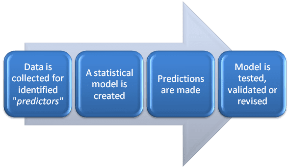
Consider three general approaches to research and modeling as employed in predictive analytics: traditional, data-adaptive, and model-dependent.

See figure 1.1. The traditional approach to research, statistical inference, and modeling begin with the specification of a theory or model.

Classical or Bayesian methods of statistical inference are employed. Traditional methods, such as linear regression and logistic regression, estimate parameters for linear predictors.

Model building involves fitting models to data and checking them with diagnostics.

We validate traditional models before using them to make predictions.

Figure 1.1. Data and models for research

When we employ a data-adaptive approach, we begin with data and search through those data to find useful predictors.

We give little thought to theories or hypotheses prior to running the analysis.

This is the world of machine learning, sometimes called statistical learning or data mining. Data-adaptive methods adapt to the available data, representing nonlinear relationships and interactions among variables.

The data determine the model. Data-adaptive methods are data-driven. As with traditional models, we validate data-adaptive models before using them to make predictions.

Model-dependent research is the third approach.

It begins with the spec-ification of a model and uses that model to generate data, predictions, or recommendations. Simulations and mathematical programming methods, primary tools of operations research, are examples of model-dependent research.

When employing a model-dependent or simulation approach, models are improved by comparing generated data with real data.

We ask whether simulated consumers, firms, and markets behave like real consumers, firms, and markets.

The comparison with real data serves as a form of validation.

It is often a combination of models and methods that works best. Consider an application from the field of financial research.

The manager of a mutual fund is looking for additional stocks for a fund’s portfolio.

A financial engineer employs a data-adaptive model (perhaps a neural network) to search across thousands of performance indicators and stocks, identifying a subset of stocks for further analysis.

Then, working with that subset of stocks, the financial engineer employs a theory-based approach (CAPM, the capital asset pricing model) to identify a smaller set of stocks to recommend to the fund manager.

As a final step, using model-dependent research (mathematical programming), the engineer identifies the minimum-risk capital investment for each of the stocks in the portfolio.

Data may be organized by observational unit, time, and space.

The observational or cross-sectional unit could be an individual consumer or business or any other basis for collecting and grouping data.

Data are organized in time by seconds, minutes, hours, days, and so on. Space or location is often defined by longitude and latitude.

Consider numbers of customers entering grocery stores (units of analysis) in Glendale, California on Monday (one point in time), ignoring the spatial location of the stores—these are cross-sectional data.

Suppose we work with one of those stores, looking at numbers of customers entering the store each day of the week for six months—these are time series data.

Then we look at numbers of customers at all of the grocery stores in Glendale across six months—these are longitudinal or panel data.

To complete our study, we locate these stores by longitude and latitude, so we have spatial or spatio-temporal data.

For any of these data structures we could consider measures in addition to the number of customers entering stores.

We look at store sales, consumer or nearby resident demographics, traffic on Glendale streets, and so doing move to multiple time series and multivariate methods.

The organization of the data we collect affects the structure of the models we employ.

As we consider business problems in this book, we touch on many types of models, including cross-sectional, time series, and spatial data models.

Whatever the structure of the data and associated models, the prediction is the unifying theme.

We use the data we have to predict data we do not yet have, recognizing that prediction is a precarious enterprise.

It is the process of extrapolating and forecasting. And model validation is essential to the process.

To make predictions, we may employ classical or Bayesian methods.

Or we may dispense with traditional statistics entirely and rely upon machine learning algorithms.

We do what works.¹ Our approach to predictive analytics is based upon a simple premise:

The value of a model lies in the quality of its predictions.

We learn from statistics that we should quantify our uncertainty.

On the one hand, we have confidence intervals, point estimates with associated standard errors, significance tests, and p-values—that is the classical way.

On the other hand, we have posterior probability distributions, probability intervals, prediction intervals, Bayes factors, and subjective (perhaps diffuse) priors—the path of Bayesian statistics. Indices such as the Akaike information criterion (AIC) or the Bayes information criterion (BIC) help us to judge one model against another, providing a balance between goodness-of-fit and parsimony.

Central to our approach is a training-and-test regimen. We partition sample data into training and test sets.

We build our model on the training set and evaluate it on the test set. Simple two- and three-way data partitioning is shown in the figure. 1.2

Figure 1.2. Training-and-Test Regimen for Model Evaluation

A random splitting of a sample into training and test sets could be fortuitous, especially when working with small data sets, so we sometimes conduct statistical experiments by executing a number of random splits and averaging performance indices from the resulting test sets.

There are extensions to and variations on the training-and-test theme.

One variation on the training-and-test theme is multi-fold cross-validation, illustrated in figure 1.3. We partition the sample data into M folds of approximately equal size and conduct a series of tests.

For the five-fold cross-validation shown in the figure, we would first train on sets B through E and test on set A. Then we would train on sets A and C through E, and test on B. We continue until each of the five folds has been utilized as a test set.

We assess performance by averaging across the test sets. In leave-one-out cross-valuation, the logical extreme of multi-fold cross-validation, there are as many test sets as there are observations in the sample.

Figure 1.3. Training-and-Test Using Multi-fold Cross-validation

Another variation on the training-and-test regimen is the class of bootstrap methods.

If a sample approximates the population from which it was drawn, then a sample from the sample (what is known as a resampling) also approximates the population.

A bootstrap procedure, as illustrated in figure 1.4, involves repeated resampling with replacement.

That is, we take many random samples with replacement from the sample, and for each of these resamples, we compute a statistic of interest.

The bootstrap distribution of the statistic approximates the sampling distribution of that statistic.

What is the value of the bootstrap? It frees us from having to make assumptions about the population distribution.

We can estimate standard errors and make probability statements working from the sample data alone.

The bootstrap may also be employed to improve estimates of prediction error within a leave-one-out cross-validation process. Cross-validation and bootstrap methods are reviewed in Davison and Hinkley (1997), Efron and Tibshirani (1993), and Hastie, Tibshirani, and Friedman (2009).

Figure 1.4. Training-and-Test with Bootstrap Resampling

Data visualization is critical to the work of data science.

Examples in this book demonstrate the importance of data visualization in discovery, diagnostics, and design.

We employ tools of exploratory data analysis (discovery) and statistical modeling (diagnostics). In communicating results to management, we use presentation graphics (design).

There is no more telling demonstration of the importance of statistical graphics and data visualization than a demonstration that is affectionately known as the Anscombe Quartet.

Consider the data sets in table 1.1, developed by Anscombe (1973). Looking at these tabulated data, the casual reader will note that the fourth data set is clearly different from the others.

What about the first three data sets? Are there obvious differences in patterns of relationship between x and y?

Table 1.1. Data for the Anscombe Quartet

Set I	Set II	Set III	Set IV
x1	y1	x2	y2	x3	y3	x4	y4
10	8.04	10	9.14	10	7.46	8	6.58
8	6.95	8	8.14	8	6.77	8	5.76
13	7.58	13	8.74	13	12.74	8	7.71
9	8.81	9	8.77	9	7.11	8	8.84
11	8.33	11	9.26	11	7.81	8	8.47
14	9.96	14	8.10	14	8.84	8	7.04
6	7.24	6	6.13	6	6.08	8	5.25
4	4.26	4	3.10	4	5.39	19	12.50
12	10.84	12	9.13	12	8.15	8	5.56
7	4.82	7	7.26	7	6.42	8	7.91
5	5.68	5	4.74	5	5.73	8	6.89

When we regress y on x for the data sets, we see that the models provide similar statistical summaries.

The mean of the response y is 7.5, the mean of the explanatory variable x is 9. The regression analyses for the four data sets are virtually identical.

The fitted regression equation for each of the four sets is ŷ = 3 + 0.5x. The proportion of response variance accounted for is 0.67 for each of the four models.

Following Anscombe (1973), we would argue that statistical summaries fail to tell the story of data.

We must look beyond data tables, regression coefficients, and the results of statistical tests.

It is the plots in figure 1.5 that tell the story. The four Anscombe data sets are very different from one another.

Figure 1.5. Importance of Data Visualization: The Anscombe Quartet

The Anscombe Quartet shows that we must look at data to understand them. An R program for the Anscombe Quartet is provided at the end of this chapter in exhibit 1.1.

Visualization tools help us learn from data. We explore data, discover patterns in data, identify groups of observations that go together and unusual observations or outliers.

We note relationships among variables, sometimes detecting underlying dimensions in the data.

Graphics for exploratory data analysis are reviewed in classic references by Tukey (1977) and Tukey and Mosteller (1977).

Regression graphics are covered by Cook (1998), Cook and Weisberg (1999), and Fox and Weisberg (2011).

Statistical graphics and data visualization are illustrated in the works of Tufte (1990, 1997, 2004, 2006), Few (2009), and Yau (2011, 2013).

Wilkinson (2005) presents a review of human perception and graphics, as well as a conceptual structure for understanding statistical graphics.

Cairo (2013) provides a general review of information graphics. Heer, Bostock, and Ogievetsky (2010) demonstrate contemporary visualization techniques for web distribution.

When working with very large data sets, special methods may be needed, such as partial transparency and hexbin plots (Unwin, Theus, and Hofmann 2006; Carr, Lewin-Koh, and Maechler 2014; LewinKoh 2014).

The R programming environment provides a rich collection of open-source tools for data visualization, including interfaces to visualization applications on the World Wide Web.

Matloff (2011) and Lander (2014) provide useful introductions to R. A graphics overview is provided by Murrell (2011).

R lattice graphics, discussed by Sarkar (2008, 2014), build upon the conceptual structure of an earlier system called S-Plus Trellis^TM (Cleveland 1993; Becker and Cleveland 1996). Wilkinson’s (2005) “grammar of graphics” approach has been implemented in the R ggplot2 and ggvis packages (Wickham and Chang 2014; Chang 2014), with programming examples provided by Chang (2013).

Cairo (2013) and Zeileis, Hornik, and Murrell (2009, 2014) provide advice about colors for statistical graphics. Ihaka et al. (2014) show how to specify colors in R by hue, chroma, and luminance.

These are the things that data scientists do:

• Finding out about. This is the first thing we do—information search, finding what others have done before, learning from the literature. We draw on the work of academics and practitioners in many fields of study, contributors to predictive analytics, and data science.
• Preparing text and data. The text is unstructured or partially structured. Data are often messy or missing. We extract features from the text. We define measures. We prepare text and data for analysis and modeling.
• Looking at data. We do exploratory data analysis, data visualization for the purpose of discovery. We look for groups in data. We find outliers. We identify common dimensions, patterns, and trends.
• Predicting how much. We are often asked to predict how many units or dollars of the product will be sold, the price of financial securities or real estate. Regression techniques are useful for making these predictions.
• Predicting yes or no. Many business problems are classification problems. We use classification methods to predict whether or not a person will buy a product, default on a loan, or access a web page.
• Testing it out. We examine models with diagnostic graphics. We see how well a model developed on one data set works on other data sets. We employ a training-and-test regimen with data partitioning, cross-validation, or bootstrap methods.
• Playing what-if. We manipulate key variables to see what happens to our predictions. We play what-if games in simulated marketplaces. We employ the sensitivity or stress testing of mathematical programming models. We see how the values of input variables affect outcomes, payoffs, and predictions. We assess uncertainty about forecasts.
• Explaining it all. Data and models help us understand the world. We turn what we have learned into an explanation that others can understand. We present project results in a clear and concise manner. These presentations benefit from well-constructed data visualizations.

Let us begin.

Exhibit 1.1. Programming the Anscombe Quartet

# The Anscombe Quartet (R)

# demonstration data from
# Anscombe, F. J. 1973, February. Graphs in statistical analysis.
#  The American Statistician 27: 1721.

# define the anscombe data frame
anscombe <- data.frame(
    x1 = c(10, 8, 13, 9, 11, 14, 6, 4, 12, 7, 5),
    x2 = c(10, 8, 13, 9, 11, 14, 6, 4, 12, 7, 5),
    x3 = c(10, 8, 13, 9, 11, 14, 6, 4, 12, 7, 5),
    x4 = c(8, 8, 8, 8, 8, 8, 8, 19, 8, 8, 8),
    y1 = c(8.04, 6.95,  7.58, 8.81, 8.33, 9.96, 7.24, 4.26,10.84, 4.82, 5.68),
    y2 = c(9.14, 8.14,  8.74, 8.77, 9.26, 8.1, 6.13, 3.1,  9.13, 7.26, 4.74),
    y3 = c(7.46, 6.77, 12.74, 7.11, 7.81, 8.84, 6.08, 5.39, 8.15, 6.42, 5.73),
    y4 = c(6.58, 5.76,  7.71, 8.84, 8.47, 7.04, 5.25, 12.5, 5.56, 7.91, 6.89))
# show results from four regression analyses with(anscombe, print(summary(lm(y1 ~ x1, data = anscombe)))) with(anscombe, print(summary(lm(y2 ~ x2, data = anscombe)))) with(anscombe, print(summary(lm(y3 ~ x3, data = anscombe)))) with(anscombe, print(summary(lm(y4 ~ x4, data = anscombe)))) # place four plots on one page using standard R graphics # ensuring that all have the same scales # for horizontal and vertical axes pdf(file = "fig_anscombe_R.pdf", width = 8.5, height = 8.5) par(mfrow=c(2,2), mar=c(5.1, 4.1, 4.1, 2.1)) with(anscombe, plot(x1, y1, xlim=c(2,20), ylim=c(2,14), pch = 19, col = "darkblue", cex = 1.5, las = 1, xlab = "x1", ylab = "y1")) title("Set I") with(anscombe,plot(x2, y2, xlim=c(2,20), ylim=c(2,14), pch = 19, col = "darkblue", cex = 1.5, las = 1, xlab = "x2", ylab = "y2")) title("Set II") with(anscombe,plot(x3, y3, xlim=c(2,20), ylim=c(2,14), pch = 19, col = "darkblue", cex = 1.5, las = 1, xlab = "x3", ylab = "y3")) title("Set III") with(anscombe,plot(x4, y4, xlim=c(2,20), ylim=c(2,14), pch = 19, col = "darkblue", cex = 1.5, las = 1, xlab = "x4", ylab = "y4")) title("Set IV") dev.off() # par(mfrow=c(1,1),mar=c(5.1, 4.1, 4.1, 2.1)) 
# return to plotting defaults 
# Suggestions for the student: 
# See if you can develop a quartet of your own, 
# or perhaps just a duet, two very different data sets 
# with the same fitted model.

This chapter is from the book